Reports
The Advanced license of Veda2.0 offers a powerful, efficient way to create reports. VEDA_BE and the Results functionality in Veda2.0 work well for interactive and even production reporting, but they have two limitations that the Reports feature removes. First, reporting variables are trapped inside tables — they cannot be controlled directly. Second, output views cannot grow new dimensions; segmentation is limited to process and commodity sets on top of the native indexes (attribute, region, time).
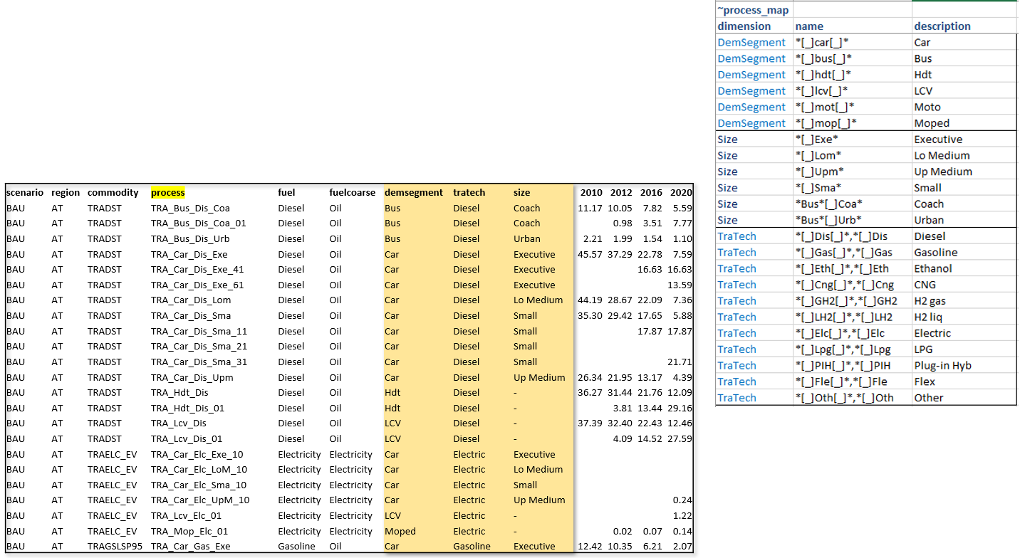
Take transportation final energy in a rich model like JRC_EU-TIMES: you may want to see energy consumption by scenario, region, fuel, mode, size, and technology. Scenario and region are separate indexes, and fuel can be managed with commodity sets — but mode, size and technology have to be expressed through process sets, which means three separate views in the table-driven approach. Reports replaces that with an Excel template in which reporting variables are defined explicitly, and any number of dimensions can be derived from process names, commodity names, regions and scenarios. The same mechanism can pull in exogenous data — historical energy balances for trend/calibration views, or population and GDP for per-capita and per-GDP metrics.
Note
Examples in this section are based on the JRC_EU-TIMES model. Further examples are in the file LMADefs-EU_TIMES.xlsm.
The Reports feature is active in Trial licenses.
Core mechanics of Report creation
The Reports menu can be used to select scenarios across models and users.
Reports are defined in one or more Excel files (analogous to the Set definitions file).
The Excel files contain tagged tables — each table begins with a tag like
~TS_Defsor~Process_Mapand is followed by a header row and data rows.- There are two main steps in building a report:
Define variables (
~TS_Defs,~TS_Ratios,~ATS_final). Each row produces one or more numbers, indexed by attribute, region, year, scenario, and optionally process/commodity/timeslice/user-constraint/vintage.Classify them with overlapping dimensions using the
_Maptags (~Varbl_Map,~Process_Map,~Commodity_Map,~Region_Map,~Timeslice_Map). Everydimensionlisted in a_Maptable becomes a new column on the report fact table, which Excel / CSV / VO / LMA can pivot, filter and slice on. The same process or commodity can carry multiple overlapping classifications (e.g. a single solar PV plant is simultaneously Tech = Solar, Sector = Power, Tech_Agg = Renewables).
All processing is region-aware: region is preserved by default in every output, and ratios computed via
~TS_Ratiosgroup by region implicitly. Region can be aggregated explicitly via~Region_Map.
Pipeline order
The order in which Veda processes tags matters when you reason about which substitutions happen first. The simplified order is:
Parse all
~TS_Defsrows.For each scenario, join the model output (
.vdfile) with the parsed variable definitions. Applyshow_meper-row retention (dimensions not listed are aggregated away). Substitute<c>/<pa>/<pc>unit placeholders. ApplyWAttributeweighted averages.Build trade-flow variables from
~Geolocation(and electricity-grid trade flows from~tradeflow_imp/~tradeflow_exp).Apply unit conversion from
~UnitConvso~TS_Ratiossees converted units.Process
~TS_Ratiosrows (numerator/denominator weighted averaging, ratio or product, parent-region roll-up).Apply dimension classifications (
~Varbl_Map,~Process_Map,~Commodity_Map,~Region_Map,~Timeslice_Map). Eachdimensionproduces a new column on the fact table.ignoreon the~TS_Defsrow suppresses_Mapprocessing for the listed dimensions.Move per-scenario tables into the main
lma_dtsreporting table.~ATS_finaldirect injection.System-wide
~UnitConversion(fromSysSettings).~Languageprocessing (translations of names/labels).
Defining variables (~TS_Defs)
The ~TS_Defs tag is the core of Reports. Each row defines one output variable from a combination of attribute,
process and commodity filters, plus optional timeslice and user-constraint qualifiers. The standard pattern is
one variable per row, with a fixed ``Name`` — the classifications and aggregations that the report consumer cares
about are added downstream by the _Map tags (see the next section). Trying to encode classifications in the
variable name itself is a legacy approach and is not recommended for new work; see Legacy: name embedding via sets.
Column reference (~TS_Defs)
Column |
Recognised aliases |
Meaning |
|---|---|---|
|
|
The TIMES output attribute the variable is built on (e.g. |
|
|
Weighting attribute for dynamic weighted averages. When set, the variable’s value is multiplied by this attribute’s value and the attribute’s value is stored as |
|
|
Comma-separated list of regions this variable applies to. Empty = all regions. |
|
|
Comma-separated list of periods (milestone years). Empty = all periods. |
|
|
Comma-separated list of vintages. Empty = all vintages. |
|
aliases include |
Process filter columns (set, name, description, commodity-in, commodity-out). Same semantics as in Veda’s process filtering. Wildcards ( |
|
aliases include |
Commodity filter columns (set, name, description). Wildcards and exclusions supported. |
|
|
Output unit. May contain placeholders |
|
|
Comma-separated timeslice list. Empty / |
|
|
Comma-separated user-constraint list. Also carries the |
|
|
Output variable name. For Sankey-specific naming with placeholders like |
|
|
Short and long descriptions of the variable. |
|
|
Dimensions to retain in the output. Any combination of |
|
|
Dimensions whose |
|
|
Restrict the variable to topology-valid (process, commodity) pairs. |
|
aliases |
Connector words ( |
|
Same as above, for commodity filters. |
show_me vs. ignore — two different controls
These two columns are often confused, but they control different things and operate on different dimension sets.
show_me(aliasgroup_by) controls per-row retention of the raw model dimensions. Codes:p(process),c(commodity),t(timeslice),u(user constraint),v(vintage). If a code is present, that dimension appears on each row of the output; if not, the variable is aggregated across that dimension. Leavingshow_meempty means the variable is fully aggregated — one row per (region, year, scenario).ignore(aliasdiscard/agg_across) is not another aggregation control —show_mealready does that.ignoreis a separate setting that tells the pipeline to suppress ``_Map`` classification for the listed dimensions on this variable. Codes:p,c,r,t— exactly the four dimensions that have a corresponding_Maptag. Useignorewhen a variable doesn’t make sense to classify on a particular dimension.
When to reach for each:
Want a variable with no per-process detail? Leave
show_meempty (the default). Don’t touchignore.Want a variable to show per-process detail? Put
pinshow_me.Want a variable to skip the ``Fuel`` / ``Fuel_Agg`` classifications produced by ``~Commodity_Map``? Put
cinignore. (Common for variables that are inherently fuel-aggregated already, where carrying per-commodity classification would be misleading.)Want a variable to skip the ``Region_WEO`` etc. classifications from ``~Region_Map``? Put
rinignore. (Common for variables that already aggregate across regions, or for global totals.)
The two columns are independent — they can be empty, set together, or set to different combinations.
Dynamic weighted averages with WAttribute
WAttribute turns a variable into a weighted average that aggregates correctly across processes, commodities,
regions and scenarios. For each row that has a non-empty WAttribute, Veda also reads the weighting attribute’s
values, multiplies the main attribute’s value by the weight, stores the weight in val~den, and drops rows where
the weight is null or zero.
This is the recommended way to build utilization factors, efficiencies, prices and emission intensities — anything that needs to behave correctly under aggregation. A worked example ships with the Veda Adv Demo model.
Note
Earlier versions of Veda computed certain ratios (CO2 intensity by DEM, capacity factor, efficiency by
DEM) automatically based on naming conventions in the output variables. That mechanism has been deprecated and is
no longer active in the report pipeline. Use WAttribute for any new weighted-ratio variable.
User-constraint reporting variables
Setting Attribute = User_con on a ~TS_Defs row turns the user-constraint values themselves into a report
variable. This is the standard pattern for reporting drivers that the model carries as user constraints — population,
GDP, demand projections, sectoral indicators — and is used heavily in production models. A typical pattern:
Attribute | Unit    | Name
User_con  | b$      | rep_GDP
User_con  | b$      | rep_GDPIND
User_con  | b$      | rep_GDPSER
User_con  | million | rep_POP
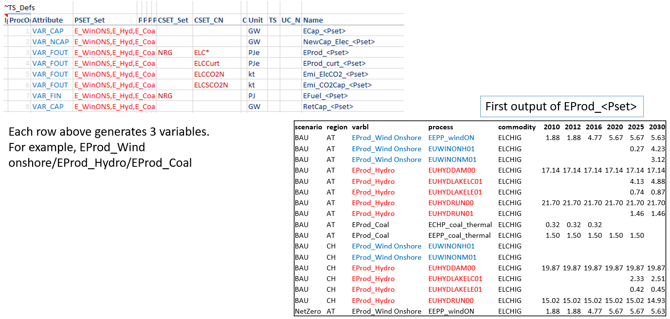
Legacy: name embedding via sets
Older report definitions encoded classifications directly into the variable name using the placeholders <Pset>,
<Cset>, <PName>, <CName>, paired with the lookup tables ~PSet_Map, ~CSet_Map, ~PName_Map,
~CName_Map:
~TS_Defs                                       ~PSet_Map
Attribute | PSET_Set    | Name                 Pset   | Desc | Ldesc
VAR_FOUT  | E_Coal      | EProd_<Pset>         E_Coal | Coal | Coal
VAR_FOUT  | E_Gas       | EProd_<Pset>         E_Gas  | Gas  | Gas
The row with PSET_Set = E_Coal produced the variable EProd_Coal, the row with E_Gas produced
EProd_Gas, and so on.
This mechanism has been completely superseded by the ``_Map`` aggregation tables. The _Map approach is more
expressive (the same process can participate in multiple overlapping classifications), keeps variable names stable,
and lets downstream tools pivot on classifications cleanly. The placeholder mechanism is still parsed for backward
compatibility, but should not be used for new work.
Aggregations and classifications (the _Map tags)
This is where Reports gets most of its expressive power. The five _Map tags — ~Varbl_Map, ~Process_Map,
~Commodity_Map, ~Region_Map, ~Timeslice_Map — attach named classifications to processes, commodities,
regions, variables and timeslices. Every dimension listed in a _Map table becomes a new column on the report
fact table.
The overlapping-subsets pattern
The single most important property of the _Map tags is that classifications can overlap freely. Unlike the
legacy set-membership approach (where a process belongs to exactly one PSET_Set per slot), _Map tables let the
same process / commodity / region appear in any number of classifications simultaneously, on different dimensions.
For example, a coal-fired power plant can be classified as all of these at once:
Sector = Power-utilTech = CoalTech_Agg = ThermalTech_CCS_flag = Without CCSRegion_WEO = North America
A natural-gas combined-cycle plant might share four of those five values, differing only on Tech = Gas. A
coal-with-CCS plant might share four of five, differing only on Tech_CCS_flag = With CCS. Each report consumer
can pivot or filter on whichever dimension they need without the others getting in the way.
Within a single dimension (e.g. Tech), the standard override rule applies — later declarations win, so a broad
pattern can be listed first and then specialised below.
How a _Map row works
Every _Map table has the same core columns plus a tag-specific set of filter columns:
Core column |
Meaning |
|---|---|
|
The name of the classification this row contributes to. Becomes a column on the output fact table. Multiple rows with the same |
|
A name pattern (with wildcards |
|
The classification value placed in the dimension column. (E.g. for a row with |
|
Long description, for localisation / UI labelling. |
The process- and commodity-specific _Map tags also accept the full set of process / commodity filter columns
that ~TS_Defs accepts (pset_set, pset_pn, pset_pd, pset_ci, pset_co, plus the c_* and
t_* variants and the _andor connectors). This lets the classification be defined by set membership, by
commodity flows (in/out), or by any combination — and is what makes overlapping classifications easy.
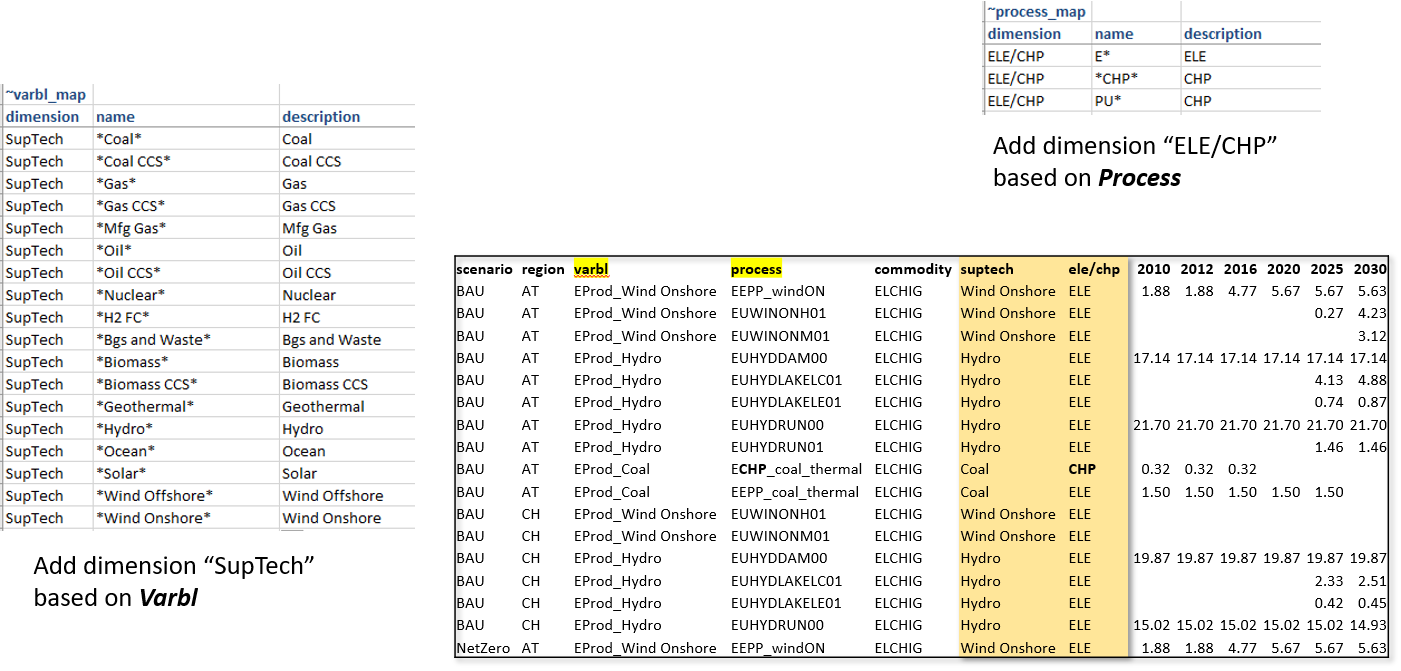
~Process_Map
Classifies processes. Supports all process filter columns.
Typical dimensions: Tech, Tech_Agg, Sector, sub_sector, sector_weo, Supply_route,
country, En_service.
A real example from a production model — the Tech dimension for power-generation technologies, combining process
set membership with commodity flows to pick out the right subsets:
~Process_Map
dimension | name           | description     | pset_set | pset_ci         | pset_co
Tech      |                | Bio             | ELE,CHP  | ???BSL,???BIO   | -CO2Captured*
Tech      |                | Coal            | ELE,CHP  | ???COA          | -CO2Captured*
Tech      |                | Gas             | ELE,CHP  | ???NGA          | -CO2Captured*
Tech      |                | Geothermal      | ELE,CHP  | ???GEO
Tech      |                | Nuclear         | ELE,CHP  | ???NUC
Tech      |                | Solar           | ELE,CHP  | ???SPV,???STH,ELC_spv_*
Tech      | *WON*,*WINONS* | Wind-Onshore    | ELE,CHP  | ???WIN,ELC_Won_*
Tech      | *WOF*,*WINOFS* | Wind-Offshore   | ELE,CHP  | ???WIN,ELC_Wof_*
Tech      |                | Bio (CCS)       | ELE,CHP  | ???BSL,???BIO   | CO2Captured*
Tech      |                | Coal (CCS)      | ELE,CHP  | ???COA          | CO2Captured*
Tech      |                | Gas (CCS)       | ELE,CHP  | ???NGA          | CO2Captured*
Three things to notice:
pset_set = ELE,CHPrestricts the classification to electricity and CHP processes.pset_ci(commodity-in) narrows further by the fuel a process consumes —???COAmatches any 3-character region prefix +COA.The CCS rows reuse the same
pset_cifilter and addpset_co = CO2Captured*(CO2-out is captured), distinguishing them from the non-CCS rows withpset_co = -CO2Captured*.
The same physical process is classified once via this single dimension. A second ~Process_Map block can give it
an orthogonal classification — for example, a coarser Tech_Agg dimension that groups Bio + Coal + Gas + Bio(CCS)
+ Coal(CCS) + Gas(CCS) under Thermal, Wind + Solar + Hydro under Renewable, and so on:
~Process_Map
dimension | description | pset_set | pset_ci
Tech_Agg  | Thermal     | ELE,CHP  | ???COA,???NGA,???BSL,???BIO,???OIL
Tech_Agg  | Renewable   | ELE,CHP  | ???SPV,???STH,???WIN,???HYD,???GEO,???TDL
Tech_Agg  | Nuclear     | ELE,CHP  | ???NUC
Tech_Agg  | Hydrogen    | ELE,CHP  | ???H2*
Tech_Agg  | Trade       | IRE
Tech_Agg  | Storage     | STG
Both dimensions land as separate columns on every output row. A pivot can show electricity production by Tech,
or roll it up by Tech_Agg, or cross-tab both.
A third ~Process_Map block can extract a sector_weo dimension purely from process-set membership, which is
typically used for WEO-style sector aggregations:
~Process_Map
dimension  | description | pset_set
sector_weo | PriSup      | s_Imports
sector_weo | PriSup      | s_Mining
sector_weo | Power       | s_Utility
sector_weo | Power       | s_Autoprod
sector_weo | Industry    | s_Industry
sector_weo | Transport   | s_Transport
sector_weo | Buildings   | s_Commercial
sector_weo | Buildings   | s_Residential
sector_weo | Hydrogen    | s_Hydrogen
sector_weo | Non-Energy  | s_Industry_NE
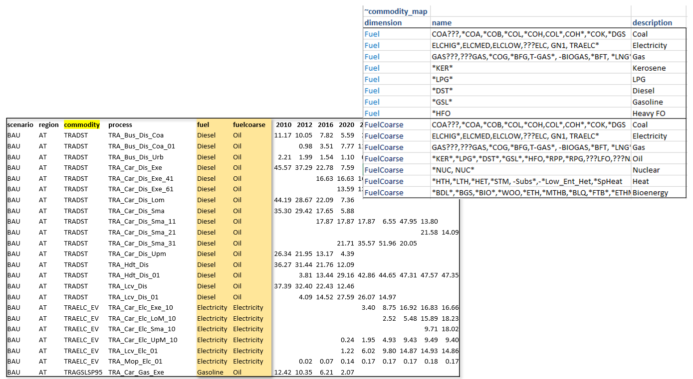
~Commodity_Map
Classifies commodities. Supports all commodity filter columns. Typical dimensions: Fuel, Fuel_Agg,
en_type, commtype, sector_c.
The Fuel / Fuel_Agg pair is the canonical example of overlapping classifications on commodities — a
fine-grained dimension and a coarser one, both present on every output row:
~Commodity_Map
dimension | name                  | description     | cset_set
Fuel      | *ELC*                 | Electricity
Fuel      | ELCCurt               | Int. Elec
Fuel      | *H2*,-[_]*            | Hydrogen
Fuel      | *HET*                 | Heat
Fuel      | *OIL*,???RPP,???RFG   | Oil
Fuel      | *GAS*,*NGA*           | Gas
Fuel      | *COA*                 | Coal
Fuel      | ???DST                | Diesel
Fuel      | ???GSL                | Gasoline
Fuel      | ???LNG                | LNG
Fuel      |                       | Biomass         | ALLBIO

Fuel_Agg  |                       | Solar           | ALLSOL
Fuel_Agg  |                       | Wind            | ALLWIN
Fuel_Agg  |                       | Hydro           | ALLHYD
Fuel_Agg  |                       | Biomass         | ALLBIO
Fuel_Agg  |                       | Nuclear         | ALLNUC
Fuel_Agg  |                       | Grid Elec       | ALLELC
Fuel_Agg  |                       | Gas             | ALLGAS
Fuel_Agg  |                       | Coal            | ALLCOAL
Fuel_Agg  |                       | Heat            | ALLHEAT
Fuel_Agg  |                       | Oil crude+NGL   | ALLOILCrd
Fuel_Agg  |                       | Oil prod.       | ALLOILprd
Fuel_Agg  | -[_]*                 | Hydrogen        | ALLH2
Note how Fuel uses name-pattern matching (*ELC*, ???DST, *OIL*) while Fuel_Agg uses set
membership (cset_set = ALLSOL etc.). Both yield independent classification columns on every output row.
Tip
As with INS tables in Veda, later declarations override earlier ones within the same dimension. Declarations
on different dimensions are independent and do not override each other. To list a broad pattern and then specialise
within a dimension: write the broad pattern first and the specific ones below. Example:
OIL* | Oil other; OILDST | Diesel; OILGSL | Gasoline.
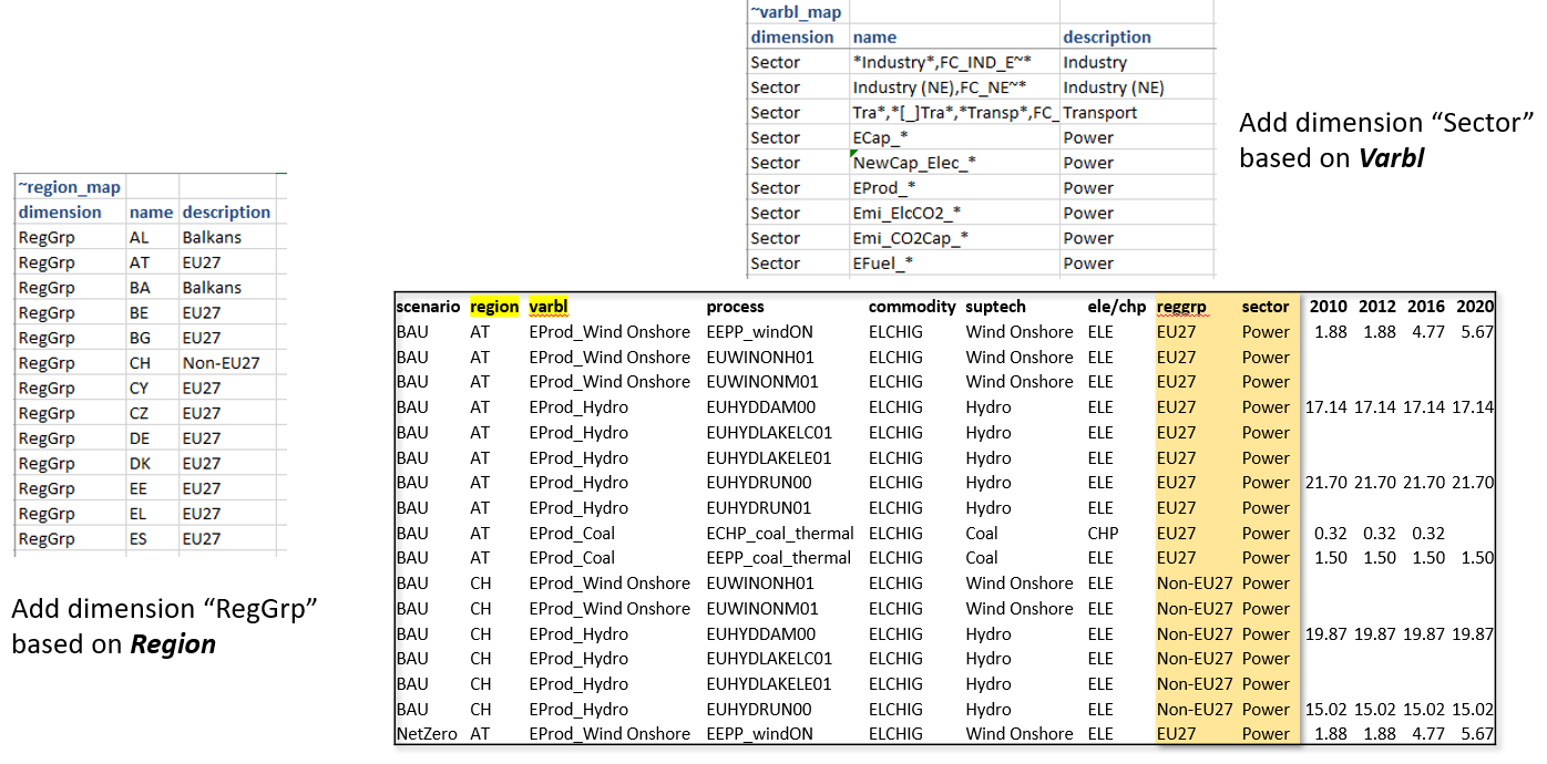
~Varbl_Map
Classifies output variables. Typical dimensions: attribute (a high-level grouping shown at the top of the
report viewer), source/use, CostType, Emi/Cap.
~Varbl_Map
dimension | name                                                          | description
attribute | *GDP*,*popu*,*percap*,*househo*,-rep*                         | Macro Indices
attribute | TFC[_]*,*[_]FE[_]*,Fin E[_]*,-*[_]IND[_]*,-*[_]Fuels[_]*,...  | Final energy
attribute | Pri_Prod*,Pri_Imp*,Pri_Exp*,PE[_]*,PriE*,Pri E*               | Primary En and Trade
attribute | Elec*_Prod                                                    | Elec Generation
attribute | Fuel_con*                                                     | Fuel Consumption
attribute | Capacity*                                                     | Capacity
attribute | CO2_emi*,CO2_cap*                                             | Emissions
attribute | Power*                                                        | Power
attribute | Prices                                                        | Prices
attribute | Cost*                                                         | Sector Costs

source/use | *[_]Agri          | Agri
source/use | *[_]Commercial    | Commercial
source/use | *[_]Residential   | Residential
source/use | *[_]Industry      | Industry
source/use | *[_]Transport     | Transport
source/use | *[_]Thermal Elec  | Thermal Elec
source/use | *[_]Thermal CCS   | Thermal CCS
source/use | *[_]Ren Elec      | Ren Elec
source/use | *[_]Bio Ref       | Bio Ref
source/use | *[_]Trade         | Trade
source/use | *[_]Extraction    | Extraction
~Region_Map
Region → grouping. Commonly used for WEO regions, OECD vs. non-OECD, EU-27 vs. EFTA, or any partition of model regions.
~Region_Map
Dimension  | Name         | Description
Region_WEO | Africa_North | Africa
Region_WEO | Africa_South | Africa
Region_WEO | Asia_Cen     | Eurasia
Region_WEO | Asia_Dev     | Asia Pacific
Region_WEO | Brazil       | C&S America
Region_WEO | Canada       | North America
Multiple Dimension values give a region multiple grouping memberships — e.g. Region_WEO, Region_OECD,
Region_Continent can all coexist as separate columns.
~Timeslice_Map
Same shape, for timeslices: dimension, name, description, ldesc. Used to roll up high-resolution
timeslices to seasons / day-vs-night / annual.
Combining classifications across maps
Because every _Map row contributes one or more columns to the same output fact table, the report consumer ends
up with a rich, denormalised view: one row per (scenario, region, year, variable, …) carrying all the classification
columns from every _Map table. Pivoting on Tech_Agg and Fuel simultaneously is a single Excel operation.
Ratios and derived variables (~TS_Ratios)
The ~TS_Ratios tag derives new variables from existing ones by combining a numerator and a denominator
variable. By default the operation is division (num / den), but setting multiply = y switches it to
multiplication (num × den). This is how shares, intensities, per-capita metrics, fuel-blend decompositions and
unit conversions involving two variables are expressed.
Internally, Veda first computes a weighted average of both the numerator and denominator at the grouping level required by the row, then joins the two and applies the requested operation. Region, year, scenario and the standard scenario keys are always part of the grouping — region grouping is the default and does not need to be requested.
Column reference (~TS_Ratios)
Column |
Type |
Meaning |
|---|---|---|
|
integer (0/1) |
When |
|
varchar |
Numerator variable name (must already exist as a |
|
varchar |
Denominator variable name. |
|
varchar |
Name of the derived output variable. |
|
varchar |
Output unit. Supports |
|
varchar |
Dimensions to retain in the weighted-average num/den groupings. Any combination of |
|
varchar |
Controls handling of regions/keys where one side has no match. |
|
varchar |
Dimensions on which to join numerator and denominator, and which are then preserved on the output. Combination of |
|
varchar |
Empty (default) → divide |
|
varchar |
Long description. |
The implicit “group by region”
Region is always part of the grouping for both numerator and denominator. There is no column to turn this off —
region is always there. This is intentional: almost every meaningful ratio is region-specific (fossil share,
generation efficiency, emission intensity). To produce a single aggregate across a group of regions, use
~Region_Map.
Adding segments via include_dim
To get a ratio at a finer level than region — by commodity, by process, by timeslice — list the dimensions in
include_dim. The numerator and denominator are joined on those dimensions, and they are kept as columns in the
output. include_dim = c produces a ratio per commodity; pc per process × commodity; and so on.
include_dim and show_me are usually set to the same value — the dimensions you want preserved are also the
dimensions you want to join on. Use different values only when you have a specific reason (e.g. you want to weight on
a dimension you don’t want to join on).
A real example — capacity factor and efficiency
From a production model:
~TS_Ratios
var_num    | var_den         | Name             | Unit    | show_me | include_null | include_dim
Elec_act   | Capacity_Elec   | Capacity_factor  | Twh/GW  | p       | y            | p
H2_Prod    | Capacity_H2     | Capacity_factor  | PJ/GW   |         | y            | p
Elec_Prod  | Fuel_cons_power | Efficiency       | Twh/PJ  |         |              | p
H2_Prod    | Fuel_cons_H2    | Efficiency       | %       |         |              | p
Capacity_factoris built per process (include_dim = p) so each technology gets its own capacity factor.include_null = yis the positive form of “use the default LEFT join” — capacity rows are preserved even if no production exists, and the ratio reads as zero in that case.
Multiplication vs division
Setting multiply = y flips the operation from division to multiplication. The typical use is decomposing one
variable using a share or fraction defined as a second variable:
Fossil_share×Petrol_total→Petrol_fossilEfficiency×Capacity→Effective_capacityPop_growth_factor×GDP_2020→GDP_projection
For multiplication the den ≠ 0 filter is dropped (num × 0 = 0 is a valid result). The val~den weight on
the output is set to NULL, because the result is no longer a ratio that needs to carry its denominator forward for
downstream weighted averaging.
The scalar = 1 case
To divide a process-level variable (e.g. process-by-process emissions) by a region-level scalar (e.g. national GDP)
to get per-GDP intensities for each process: set scalar = 1. The scalar variable is defined with process = '-'
in its source. Veda then:
does not join on
process(the denominator has no process dimension);keeps
processon the output so the per-process intensities are reported.
This is the standard pattern for rep_totco2 / rep_POP → CO2 per capita, rep_totco2 / rep_GDP → CO2/GDP, and
similar macro-normalised metrics.
Unit conversion in the output
When unit contains <unit_num> or <unit_den>, the placeholders are replaced with the actual units of the
numerator and denominator variables at runtime. After ~TS_Ratios processing, a unit-conversion pass runs on the
derived variables so ~UnitConv rules apply to them just as they do to ~TS_Defs variables.
Behaviour when one variable is defined in only some regions
A common situation: a fuel-blend share, a tax rate, or a regional adjustment factor is defined for only a subset of
regions, while the variable it is combined with exists everywhere. Two columns govern the output: include_null
and the order in which the variables appear in var_num / var_den.
With the default LEFT JOIN (include_null empty or y):
For division (
num / den), all denominator rows are preserved. In a region where the numerator is missing, the result is reported as zero.For multiplication (
multiply = y), all numerator rows are preserved. In a region where the denominator is missing, the result is reported as zero.So with multiplication, if the share/ratio (defined in fewer regions) is placed in
var_den, every region where the total quantity is reported will appear in the output — with zero for the regions where the share is undefined. If the share is placed invar_numinstead, only the regions where the share is defined will appear.
With include_null = n the join becomes INNER: only region/year combinations where both sides are present
survive. Use this to drop regions where the ratio is not meaningful, rather than to report zeros for them.
A second option, often cleaner, is to extend the share variable’s definition to cover all regions — typically with a default of 0 (so the decomposition leaves the residual untouched) or 1 (so the decomposition assigns the whole quantity to one side).
Including exogenous data (~ATS_final)
~ATS_final registers user tables that are inserted directly into the main reporting fact table (lma_dts)
after the rest of the report pipeline has run. It is the standard way to bring in historical IEA energy balances,
WEO projections, calibration overlays, or any other already-shaped data that needs to sit alongside the model output:
~ATS_Final
model | Scenario | scen     | Region        | Varbl          | Unit   | year | val      | fuel | fuel_agg   | Sector       | Region_WEO
IEA   | Hist     | Hist     | Africa_North  | CO2_emissions  | Mt CO2 | 1995 | 0.088852 | Oil  | Oil crude  | Industry     | Africa
IEA   | Hist     | Hist     | Africa_North  | CO2_emissions  | Mt CO2 | 2000 | 3.722594 | Diesel | Oil prod.| Transport    | Africa
...
Note how the source table can carry classification columns (fuel, fuel_agg, Sector, Region_WEO) that
match the dimension values produced by the _Map tags. Those values are copied straight through to the report,
so the injected rows participate in the same pivots as the model output.
How it works
Each ~ATS_final table is registered under the ATS_final tag in veda_tag_master. At report time, Veda
inspects each registered table and the central lma_dts table side by side, and for every column whose name appears
in both, the value is copied across. Source-table columns may include the canonical names — model, scen
(alias scenario), region, varbl, unit, year (alias yr), val — plus any other lma_dts
column the source chooses to populate (process, commodity, timeslice, userconstraint, vintage,
sow, val~den, and any classification columns added by the _Map tags such as Fuel, Tech,
sector_weo, Region_WEO, etc.).
Any required lma_dts column missing from the source table is filled with a default:
scenario,model,user,studyandscen_model_frameworkfall back to the first row ofscenario_master(the first scenario in the report) — or to-if no scenario is registered.All other process/commodity/timeslice/UC/vintage columns default to
-.
Because the pass runs after ~TS_Ratios and ~UnitConv, anything in an ~ATS_final table arrives in the
report as-is and is not re-aggregated, weighted or unit-converted by the standard pipeline. The user owns the row
shape and units.
Tip
Use ~ATS_final when the data is already in its final reporting shape. For exogenous variables that should
behave like every other report variable (groupings, ratios, unit conversions, weighted averages), use the simpler
~ATS tag described in “Less common tags”.
Unit conversion (~UnitConv)
~UnitConv converts the unit of a variable: where the variable’s unit matches Unit1, multiply by MultFact
and replace the unit with Unit2. Applies to both ~TS_Defs outputs and ~TS_Ratios-derived variables.
~UnitConv
Model    | Unit1     | Unit2          | MultFact
KINESYS  | kt CH4    | Mt CH4/yr      | 0.001
KINESYS  | kt CO2    | Mt CO2/yr      | 0.001
KINESYS  | kt CO2neg | Mt CO2/yr      | -0.001
KINESYS  | m$        | billion $/yr   | 0.001
KINESYS  | PJe       | Twh            | 0.27778
KINESYS  | PJ2gw     | GW             | 0.03171
The Model column scopes the rule (so different models can carry different conversion factors). Unit1 matches
case-insensitively against the variable’s current unit.
GIS trade flows (~Geolocation)
The ~Geolocation tag is a simple region → (latitude, longitude) table. Its primary role is to enable
auto-generated trade-flow variables for visualisation on maps.
~Geolocation
Region        | Lat        | Lng
UAE           | 23.424076  | 53.847818
LatAm         | -38.416097 | -63.616672
Australia     | -25.274398 | 133.775136
Bangladesh    | 23.684994  | 90.356331
Auto-generated trade-flow variables
When ~Geolocation is present and there are inter-regional exchange (IRE) processes, Veda automatically generates
three trade variables on top of the report:
trade_flows— built fromVAR_FIN(import side) andVAR_FOUT(export side) on IRE processes.trade_flows_cap— capacity of trade infrastructure (fromVAR_CAPon IRE).trade_flows_ncap— new capacity additions of trade infrastructure (fromVAR_NCAPon IRE).
Each output row carries a region_to column with the destination region, alongside region (the source). The
unit defaults to the trade commodity’s unit (or to GW? for cap / ncap if no capacity unit is set).
Electricity grid trade flows
If the report carries ~tradeflow_imp and ~tradeflow_exp variables (typically defined via ~TS_Defs rows
with a region_com column for the counterparty region), Veda generates grid_flows, grid_flows_cap and
grid_flows_ncap as a final step, with the same region_to shape.
Scenarios — ~ScenMap and ~ScenG
~ScenMap and ~ScenG provide scenario-level metadata and renaming.
~ScenMap renames model-internal scenario names (Oname) to a presentation-friendly name (Name) and adds
short and long descriptions. A production model might map dozens of internal scenario codes to readable names like
Base.SSP2, STEPS.SSP2, APS.SSP2, NZE.SSP2.
~ScenG (Scenario Generation) attaches a flexible set of classification columns to each scenario. Each column name
becomes a new dimension in the output, just like the classification columns produced by the _Map tags. Typical
~ScenG columns: Climate, SSP, Exo_price, NZYear, C_Budget, CO2Price — so a single report
can be sliced by climate scenario, SSP scenario, or any other axis the modeler chose to declare.
~ScenMap                                   ~ScenG
Oname    | Name        | Desc | Ldesc      Scen        | SSP  | Climate | Exo_price
KS~0001  | Base.SSP2   |      |            Base.SSP2   | SSP2 | Base    |
KS~0002  | STEPS.SSP2  |      |            STEPS.SSP2  | SSP2 | ESTPS   |
KS~0003  | APS.SSP2    |      |            APS.SSP2    | SSP2 | PAS     |
Multi-language support (~Language)
The ~Language tag holds translations of variable names, dimension values, region names — anything that appears in
the report and may need to be displayed in a non-English UI. The first column is name (the canonical English
label); each remaining column is an ISO 639-2 language
code (e.g. FRA, DEU, ESP, JPN, CHI) with the translated value.
~Language
name         | FRA            | DEU           | ESP                  | JPN                | CHI
Agriculture  | Agriculture    | Landwirtschaft| Agricultura          | 農業                | 农业
Asia Pacific | Asie-Pacifique | Asien-Pazifik | Asia Pacífico        | アジア太平洋地域    | 亚太地区
BF gas       | Gaz BF         | BF-Gas        | gasolina BF          | BFガス             | 高炉气体
Veda transforms the wide table into a long mapping (one row per (name, language) pair) and back into a pivoted lookup table, so downstream consumers (VO, LMA) can render the report in the chosen language.
Sankey Diagram Creation
The Reports functionality provides sophisticated capabilities for creating Sankey diagrams that visualize energy and material flows through the modeled system. Sankey diagrams are automatically generated from TIMES model results by defining source-commodity-sink relationships that VEDA processes into connected flow visualizations.
Conceptual Approach
The key to successful Sankey creation is thinking in terms of source-commodity-sink triplets. Each energy or material flow can be conceptualized as:
Source → Commodity → Sink
Examples: - Coal Mining → Coal → Power Plant - Power Plant → Electricity → Industrial Demand - Solar Farm → Electricity → Battery Storage - Battery Storage → Electricity → Residential Demand
VEDA automatically chains these triplets together when the sink of one layer becomes the source of the next layer, creating seamless flow visualizations.
Three Types of Sankey Creation
1. Set-Based Sankey Diagrams
Set-based Sankey diagrams aggregate flows using process and commodity sets, creating clean high-level visualizations with semantic naming.
Pattern: <cset description>_src/snk_<pset description>
Configuration Example:
~TS_Defs: Snk_attr=SANKEY_energy_overview
Attribute |
PSET_Set |
PSET_PN |
PSET_PD |
PSET_CI |
PSET_CO |
CSET_Set |
CSET_CN |
CSET_CD |
Unit |
TS |
UC_N |
Name |
|---|---|---|---|---|---|---|---|---|---|---|---|---|
VAR_FIN |
“ELE,CHP” |
“ALLSOL,ALLWIN,ALLHYD” |
PJ |
<cset>_src_<pset> |
||||||||
VAR_FOUT |
“DMD_IND,DMD_RES,DMD_COM” |
“ALLELC” |
PJ |
<cset>_snk_<pset> |
Process:
1. Uses PSET_Set and CSET_Set columns to specify process/commodity sets
2. Descriptions come from separate ~PSet_Map and ~CSet_Map tables
3. Creates flows between all commodity sets × process sets combinations
Generated Variables:
- Electricity_src_Renewable_Generation (from ALLSOL,ALLWIN,ALLHYD to ELE,CHP)
- Electricity_snk_Industrial_Demand (from ALLELC to DMD_IND)
- Electricity_snk_Residential_Demand (from ALLELC to DMD_RES)
Use Cases: Sector-level energy flow analysis
Set-Based Sankey Example: Whole Energy System Overview
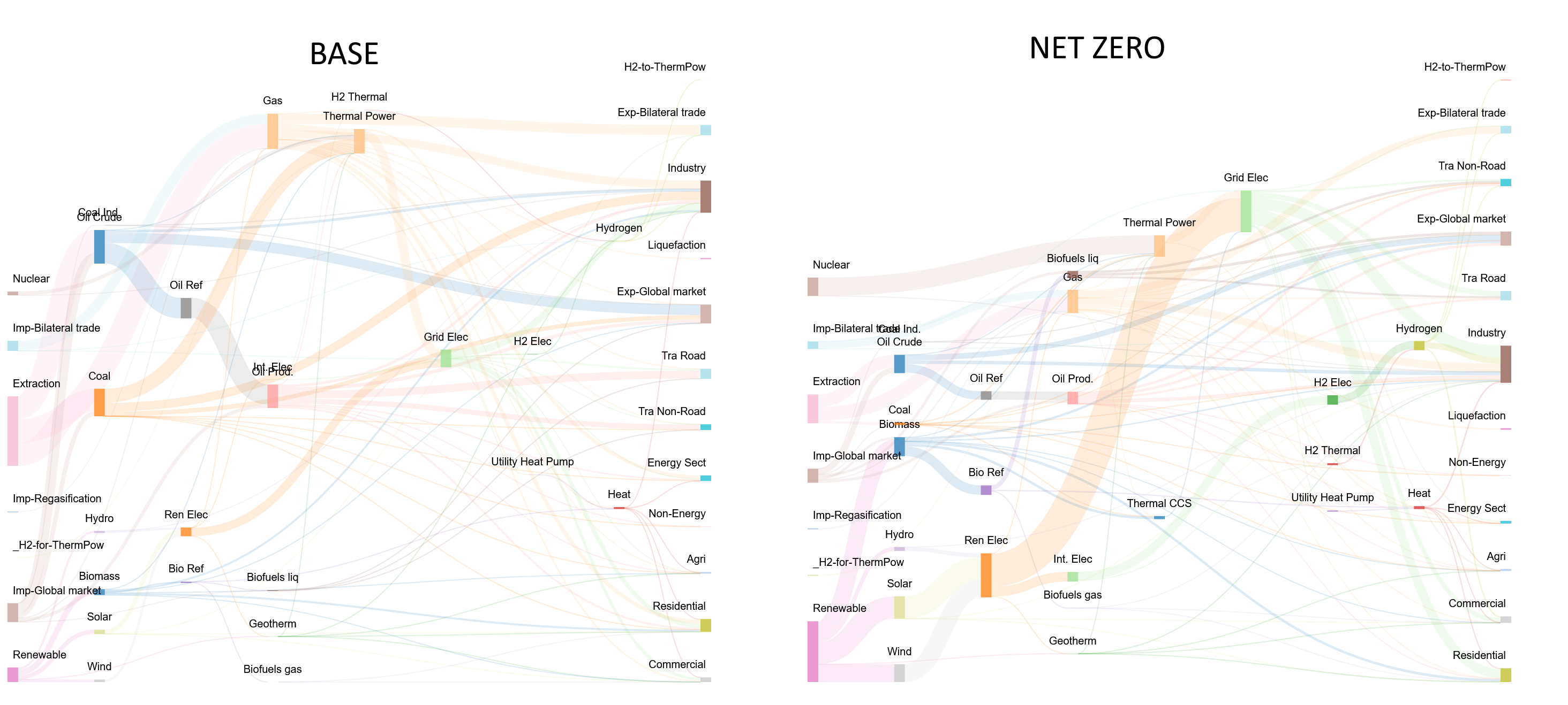
This diagram illustrates a comprehensive energy system view using set-based aggregation, showing flows from primary energy sources through conversion technologies to end-use sectors, with clean semantic naming for intuitive understanding.
2. Region-Based Sankey Diagrams
Region-based Sankey diagrams focus on inter-regional trade flows, particularly useful for gas pipelines, electricity transmission, and energy security analysis.
Pattern: <commodity>-<region>_Src/Snk_<process description>
Configuration Example:
~TS_Defs: Snk_attr=SANKEY_gas_trade
Attribute |
PSET_Set |
PSET_PN |
PSET_PD |
PSET_CI |
PSET_CO |
CSET_Set |
CSET_CN |
CSET_CD |
Unit |
TS |
UC_N |
Name |
|---|---|---|---|---|---|---|---|---|---|---|---|---|
VAR_FIN |
IRE |
*gaspip* |
GASNGA |
Pjneg |
Nat Gas-<region>_Snk_<gen_pname> |
|||||||
VAR_FOUT |
IRE |
*gaspip* |
GASNGA |
PJ |
Nat Gas-<region>_Src_<gen_pname> |
|||||||
VAR_FIN |
PRE |
GASLNG |
GASNGA |
Pjneg |
Nat Gas-<region>_Snk_<gen_pname> |
|||||||
VAR_FOUT |
PRE |
GASLNG |
GASNGA |
PJ |
Nat Gas-<region>_Src_<gen_pname> |
Process:
1. <region> placeholder gets replaced with actual region names
2. <gen_pname> generates descriptive process names
3. Pattern matching (*gaspip*) identifies relevant processes
Generated Variables:
- Nat Gas-USA_Snk_Pipeline-to-Canada (US gas export to Canada)
- Nat Gas-Russia_Src_Pipeline-to-Europe (Russian gas export to Europe)
- Nat Gas-Germany_Snk_LNG-Terminal (German LNG imports)
Use Cases: Gas pipeline networks, LNG trade flows, regional energy security, cross-border electricity trade
Region-Based Sankey Example: Natural Gas Trade Networks
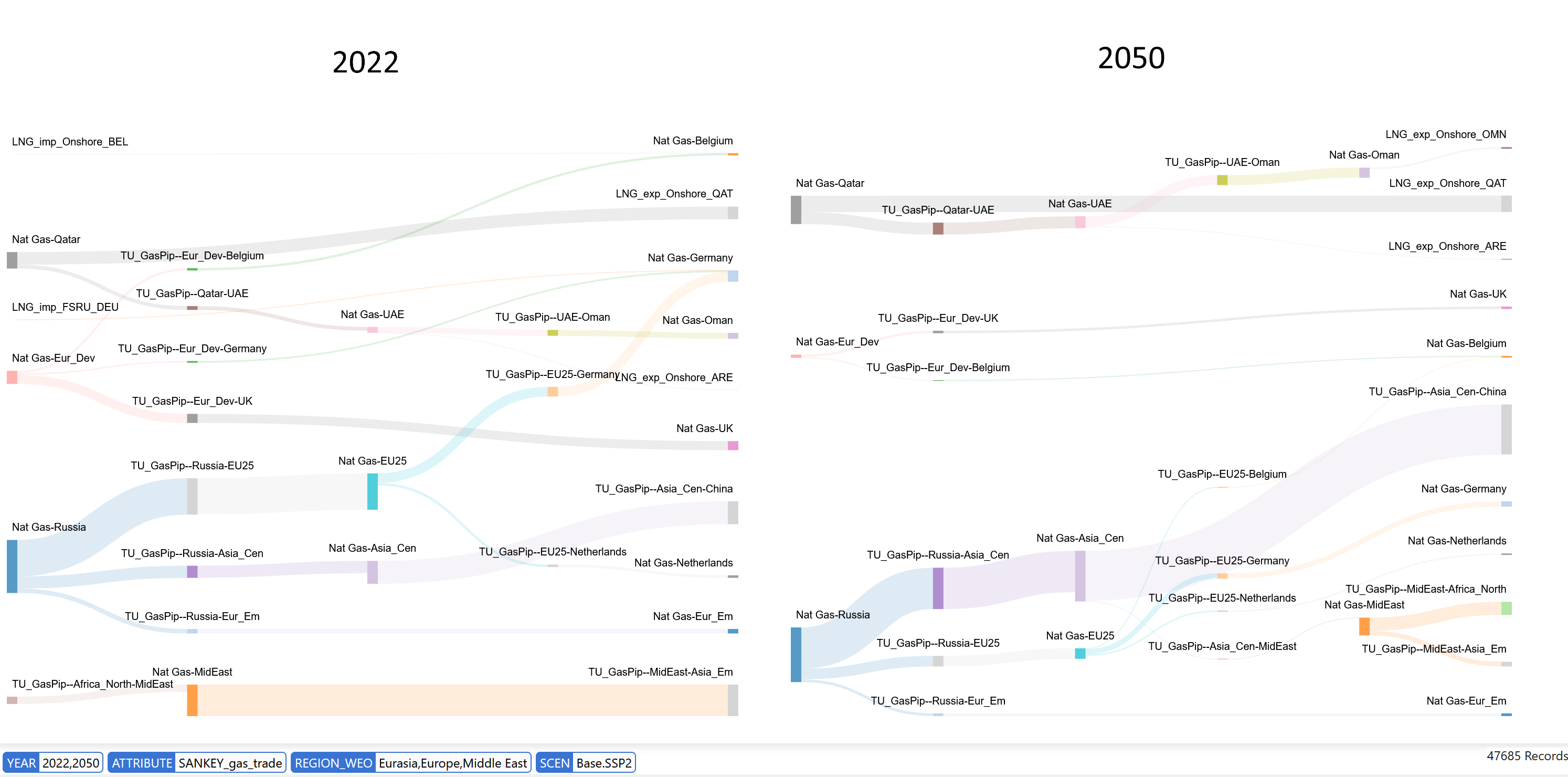
This diagram demonstrates inter-regional natural gas trade flows, showing pipeline connections and LNG terminals with region-specific naming that enables energy security and infrastructure analysis across multiple countries.
3. Granular Sankey Diagrams
Granular Sankey diagrams preserve full model detail, showing individual processes and commodities without aggregation.
Pattern: <gen_cname>_Snk/Src_<gen_pname>
Configuration Example:
~TS_Defs: Snk_attr=SANKEY_steel_detailed
Attribute |
PSET_Set |
PSET_PN |
PSET_PD |
PSET_CI |
PSET_CO |
CSET_Set |
CSET_CN |
CSET_CD |
Unit |
TS |
UC_N |
Name |
|---|---|---|---|---|---|---|---|---|---|---|---|---|
VAR_FIN |
“PRE,DMD” |
MAT |
“im_*,ind[_]*” |
Mtneg |
<gen_cname>_Snk_<gen_pname> |
|||||||
VAR_FOUT |
“PRE,DMD” |
MAT |
“im_*,ind[_]*” |
Mt |
<gen_cname>_Src_<gen_pname> |
|||||||
VAR_FIN |
IRE |
MAT |
“im_*,ind[_]*” |
Mtneg |
<gen_cname>_Snk_Export |
|||||||
VAR_FOUT |
IRE |
MAT |
“im_*,ind[_]*” |
Mt |
<gen_cname>_Src_Import |
Process:
1. Each commodity and process gets its own flow variable
2. Uses PSET_PN and CSET_CN for pattern-based selection
3. <gen_cname> and <gen_pname> use actual model names
Generated Variables:
- Iron_Ore_Snk_Blast_Furnace_Plant_01 (specific iron ore to specific plant)
- Steel_Src_Electric_Arc_Furnace_02 (specific steel from specific EAF)
- Crude_Oil_Snk_Refinery_Houston (specific crude to specific refinery)
Use Cases: Detailed industrial analysis, plant-level material flows, supply chain traceability, bottleneck identification
Granular Sankey Example: Industrial Material Flows
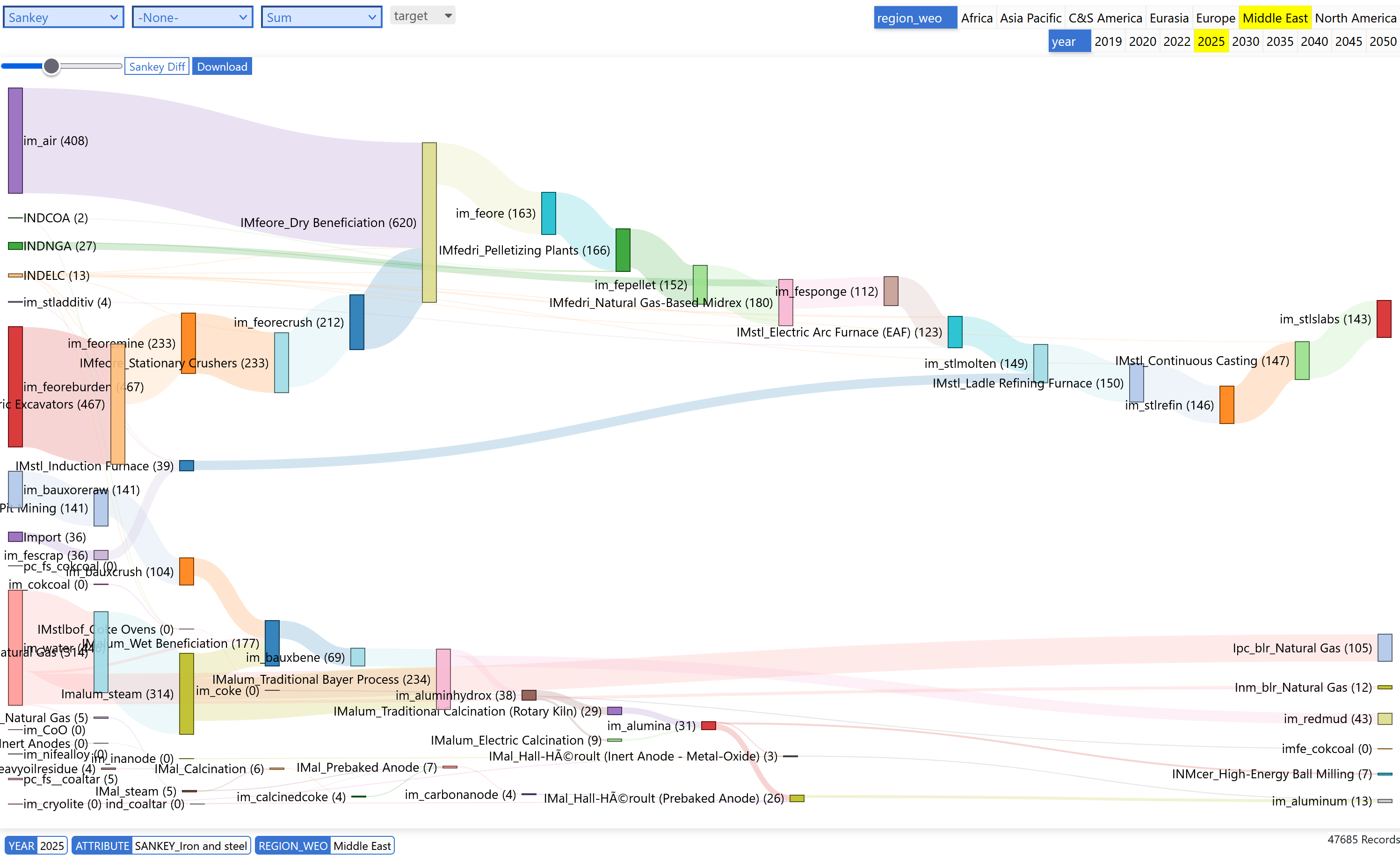
This diagram shows detailed iron and steel production flows in the Middle East region for 2025, demonstrating how granular Sankey diagrams can trace individual material streams through specific industrial processes.
Advanced Sankey Features
Flow Direction and Units
VEDA uses variable types and units to determine flow directions:
- VAR_FIN with negative units (Pjneg, ktneg) = Consumption/Sink flows
- VAR_FOUT with positive units (PJ, kT) = Production/Source flows
Pattern Matching and Exclusions
Sophisticated filtering using wildcards and exclusions:
Filter Type |
Pattern |
Description |
|---|---|---|
PSET_PN |
“*gaspip*” |
Matches all gas pipeline processes |
PSET_PN |
“MinBio*” |
Matches biomass mining processes |
PSET_PN |
“-EA_HH2*” |
Excludes hydrogen heating processes |
CSET_CN |
“-SUP*,-COAOVC” |
Excludes supply and coal processes |
Dynamic Naming with Placeholders
Flexible variable naming using placeholders:
- <cset> - Replaced with commodity set description
- <pset> - Replaced with process set description
- <region> - Replaced with region name
- <gen_pname> - Generated process name
- <gen_cname> - Generated commodity name
Automatic Flow Chaining
VEDA automatically connects flows when naming patterns match:
- Coal_snk_Power_Plant ←→ Electricity_src_Power_Plant
- Electricity_snk_Battery ←→ Electricity_src_Battery
This intelligence allows complex multi-layer Sankey diagrams to be created with minimal configuration.
Sankey Configuration Strategy
Choose Set-Based When: - Creating executive dashboards for policy makers - Showing technology competition (renewables vs. fossils) - Sector-level energy flow analysis - Clean, interpretable visualizations needed
Choose Region-Based When: - Analyzing energy security and trade dependencies - Visualizing cross-border infrastructure - Geographic context is primary concern - Regional integration analysis
Choose Granular When: - Engineering analysis of specific facilities - Supply chain optimization and bottleneck analysis - Detailed validation against real-world data - Asset-level investment decisions
Practical Design Workflow: 1. Sketch the physical system on paper 2. Identify major transformation/aggregation points 3. Define commodity flows between each point 4. Write source-commodity-sink triplets for each flow 5. Configure VEDA filters to capture these triplets 6. Let VEDA automatically chain and visualize
This approach puts energy system understanding in the user’s hands while leveraging VEDA’s automation for technical implementation.
See also
These Sankey capabilities have been used extensively in KiNESYS applications — see the Argonne NetZero World example (EU-Ukraine trade corridors) and KAPSARC OPEC oil & gas systems in the KiNESYS Applications and Impact documentation.
Viewing Reports
Veda2.0 ships with a basic report viewer that is sufficient for validating the report setup and for simple visualizations. Excel export and CSV dumps are supported, as in Results.

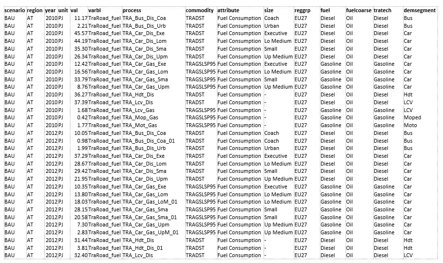
CSV output
The CSV output can be consumed in Tableau, Power BI, LMA, and similar tools:
VO gets a lot more out of Reports
VO (Veda Online) offers the core Veda-TIMES functionality via Internet browsers. Veda model folders need to reside on GitHub to be used under VO. Registered users can submit their GitHub credentials to see a list of all model folders, along with the branches, under their account. Any folder/branch can be selected to create a model. Supported functionality: Synchronize, Browse, Items view, Run manager, Results, and Reports.
See also
The _map table capabilities and Sankey diagram creation documented above have been extensively used in real-world applications
including World Bank CCDRs, corporate transition planning, and multi-model research. For concrete examples of how these features
enable interactive exploration across scenarios and regions, see the KiNESYS Applications and Impact documentation.
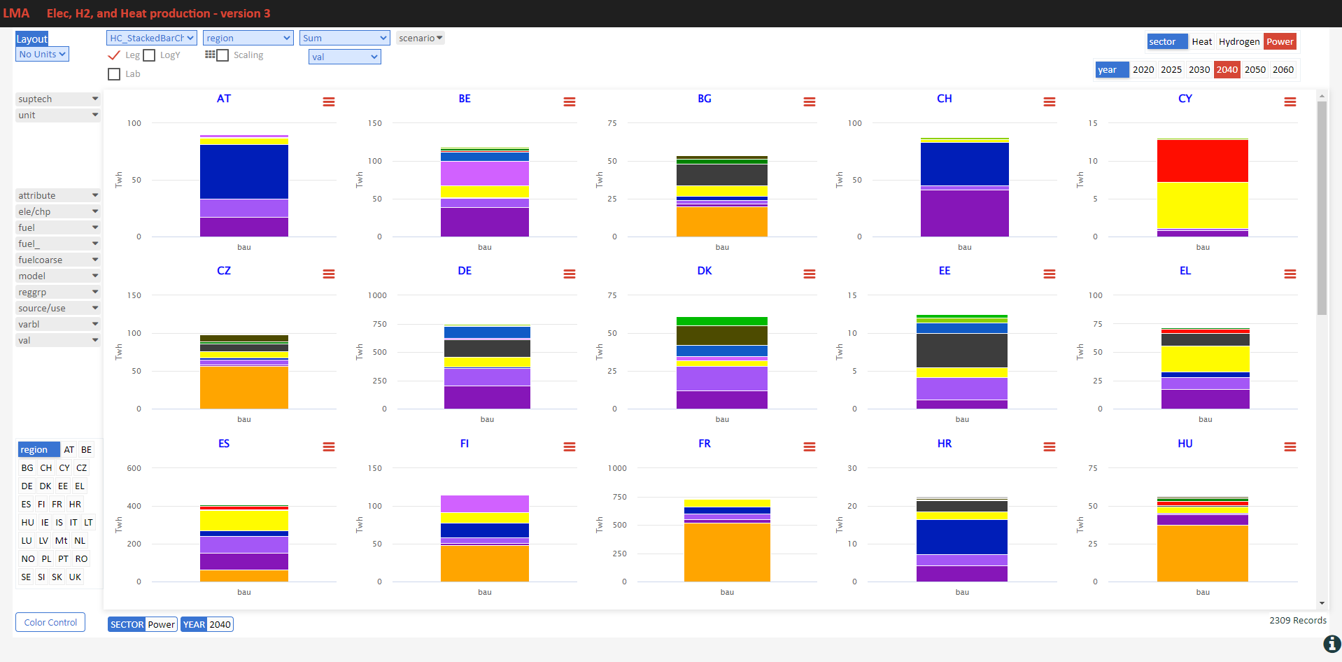
Here are some sample visualizations on the same platform that drives VO reports.
Sources and uses of main energy forms
- See it online select energy form
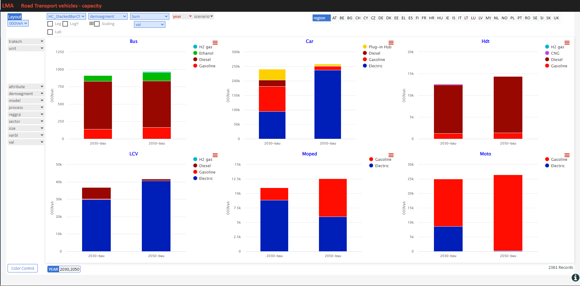
Road transport vehicles
- See it online select region
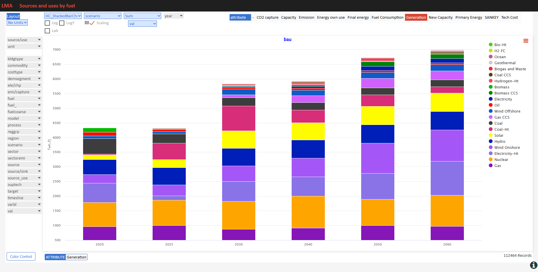
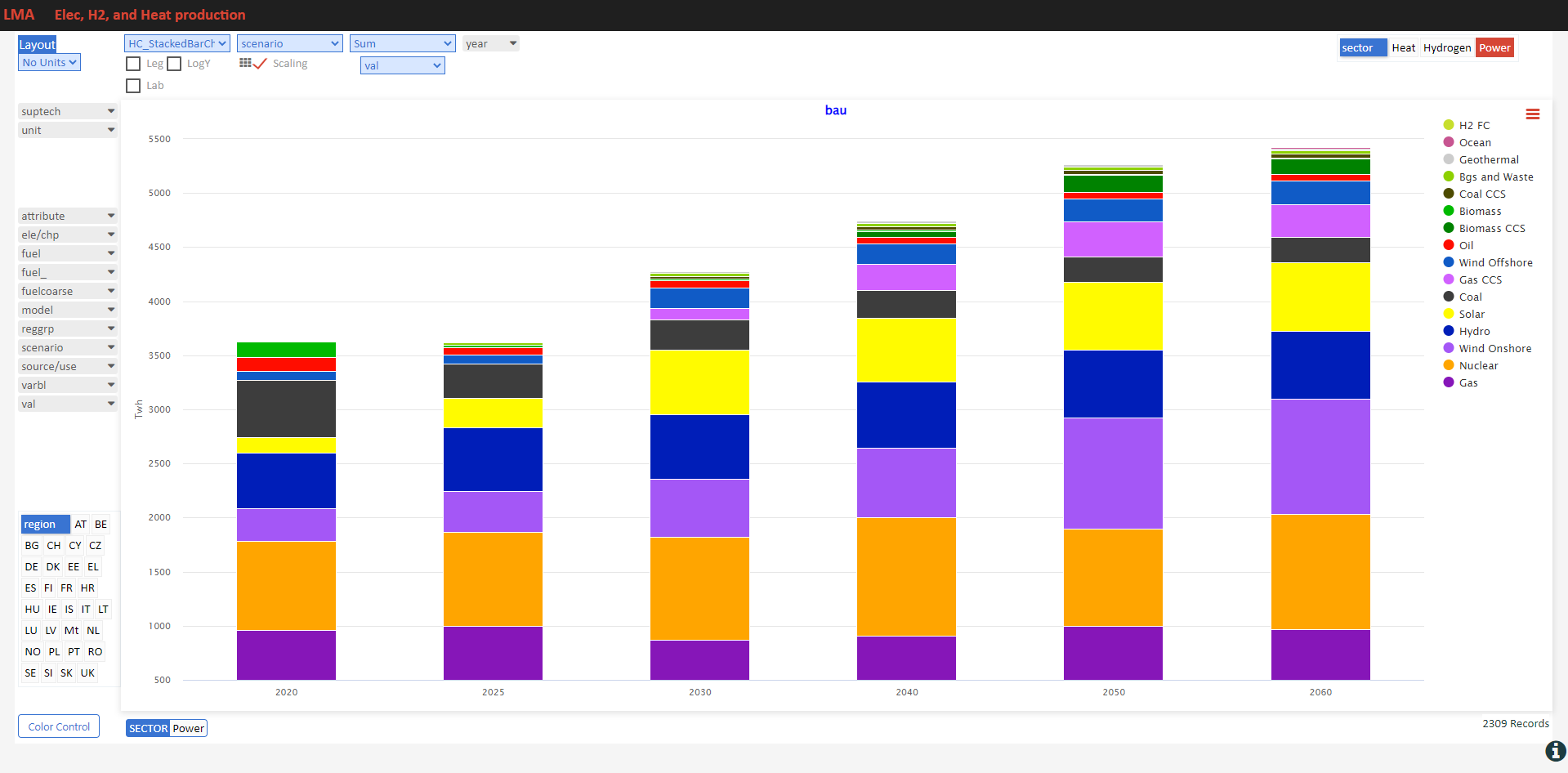
Power generation
- See it online select electricity/hydrogen/heat, and region
Power generation – alternate view
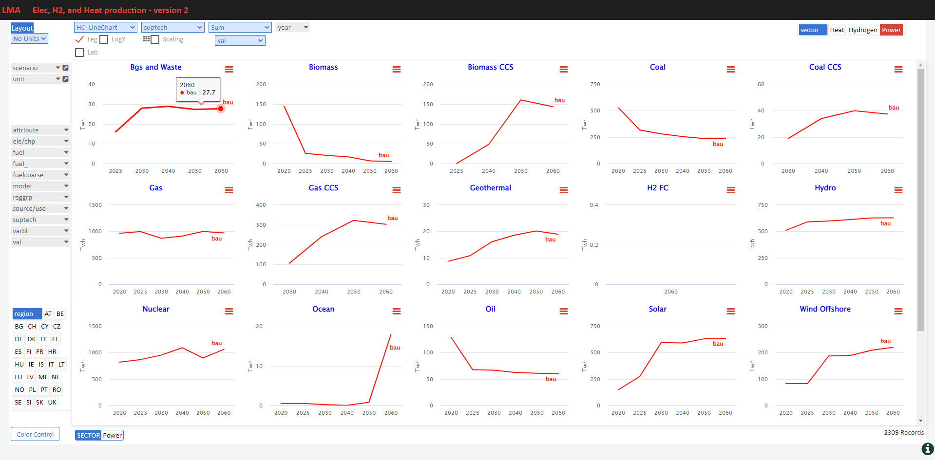
Power generation – alternate view 2